Residual Defect Estimation Model: Such a calculation can be embedded in the Residual Defect Estimation Model in which we are using, the number of introduced defects and the test effectiveness, a simple calculation results in the number of residual defects.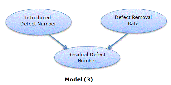
Test Estimation Model: To estimate the effort and duration for the indicated test is the main aim of the Test Estimation Model. The inputs for estimation of test effort and test duration are number of requirements and average number of people who are focusing on testing. With this model, managers can estimate the test effort and duration with the indicated test scope, which is the number of requirements here. Also a trade-off analysis for test resources can also be made using this sub-model.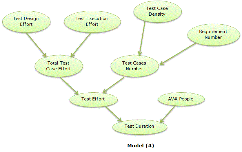
Other Commanly Used Models Are:
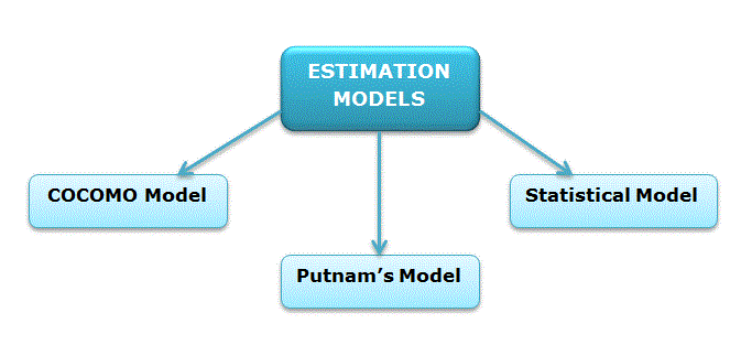
COCOMO MODEL
COCOMO Model is introduced by Barry Boehm and stand for constructive cost model which is best known and most thoroughly documented of all software cost estimation models. It provides the following three levels of models:
- Basic
- Intermediate
- Detailed
Basic COCOMO: Basic COCMO Model is good for quick, early, rough order of magnitude estimate of software cost. It does not account for differences in hardware constraints, personal quality and experience, use of modern tools and techniques, and other project attribute known to have a significant influence on software cost, which limits its accuracy. It gives an approximate estimate of the project parameters. The basic COCOMO estimation model is given by the following expressions:
- Effort Applied (E) = a(KLOC)^b [ man-months ]
- Development Time (D) = c(Effort Applied)^d [months]
- People required (P) = Effort Applied / Development Time [count]

Intermediate COCOMO: The intermediate COCOMO model takes the basic COCOMO model as its starting point which means that it is slightly different coefficients for the effort equation than the Basic model. After that it multiplies the basic estimate by an Effort Adjustment Factor which is calculated as the product of 15 multipliers (cost drivers) which take into account factors such as required product reliability, database size, execution and storage constraints, personnel aptitude, and the use of software tools. It produces better results than the Basic model because the user supplies settings for cost drivers that determine the effort and duration of the software projects.
Detailed COCOMO: A major shortcoming of both the basic and intermediate COCOMO models is that they consider a software product as a single homogeneous entity. However, most large systems are made up several smaller sub-systems. These sub-systems may have widely different characteristics.
The Detailed COCOMO model differs from the Intermediate COCOMO model in that it uses effort multipliers for each phase of the project. These phase dependent effort multipliers yield better estimates because the cost driver ratings may be different during each phase.
Barry Boehm suggested that a detailed model would provide a cost estimate to the accuracy of ± 20 % of actual value.
This model may be applied to three classes of software projects as given below:
- Organic: Small size project. A simple software project where the development team has good experience of the application
- Semi-detached: An intermediate size project and project is based on rigid and semi-rigid requirements.
- Embedded: The project developed under hardware, software and operational constraints. Examples are embedded software, flight control software.
PUTNAM'S MODEL
A dynamic multivariate model of the software development process named as "Putnam's model is developed by L. H. Putnam which is based on the assumption that distribution of effort over the life of software development is described by the Rayleigh-Norden curve.
P = Kt exp(t2/2T2) / T2
P = No. of persons on the project at time 't'
K = The area under Rayleigh curve which is equal to total life cycle effort
T = Development time
The Rayleigh-Norden curve is used to derive an equation that relates lines of code delivered to other parameters like development time and effort at any time during the project.
S = CkK1/3T4/3
S = No. of delivered lines of source code (LOC)
Ck = State-of-technology constraints
K = Life cycle effort in man-years.
T = Development time.
STATISTICAL MODEL
From the data of a number of completed software projects, C.E. Walston and C.P. Felix developed a simple empirical model of software development effort with respect to number of lines of code. In this model, LOC is assumed to be directly related to development effort as given below:
E = a Lb
Where L = Number of Lines of Code (LOC)
E = total effort required
a and b are parameters obtained from regression analysis of data. The final equation is of the following form:
E = 5.2 L0.91
The productivity of programming effort can be calculated as
P = L/E
Where P = Productivity Index
Automated Tools For Estimation
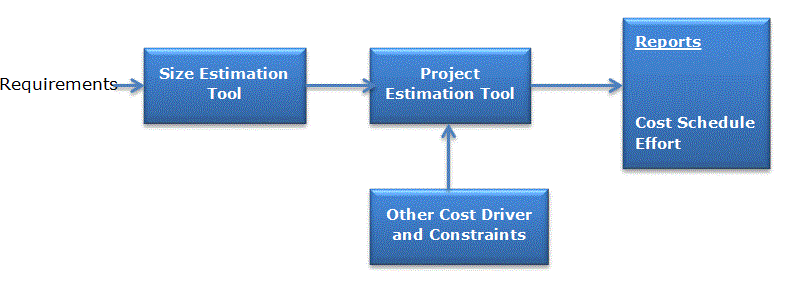
After learning all these models for software project estimation, now it's time to think of software that implements these models. This is what exactly the automated estimation tools do. These estimation tools, which estimate cost and effort, allow the project managers to perform "What if analysis". Estimation tools may only support size estimation or conversion of size to effort and schedule to cost.
There are more than dozens of estimation tools available. But, all of them have the following common characteristics:
- Quantitative estimates of project size (e.g., LOC).
- Estimates such as project schedule, cost.
- Most of them use different models for estimation.
Nipun Tomar (c-sharpcorner.com)
Back to part 2

